Methods
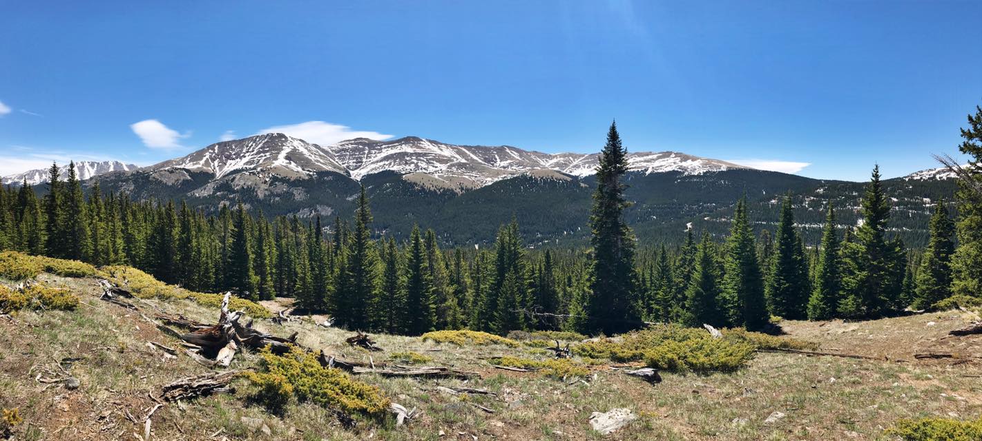
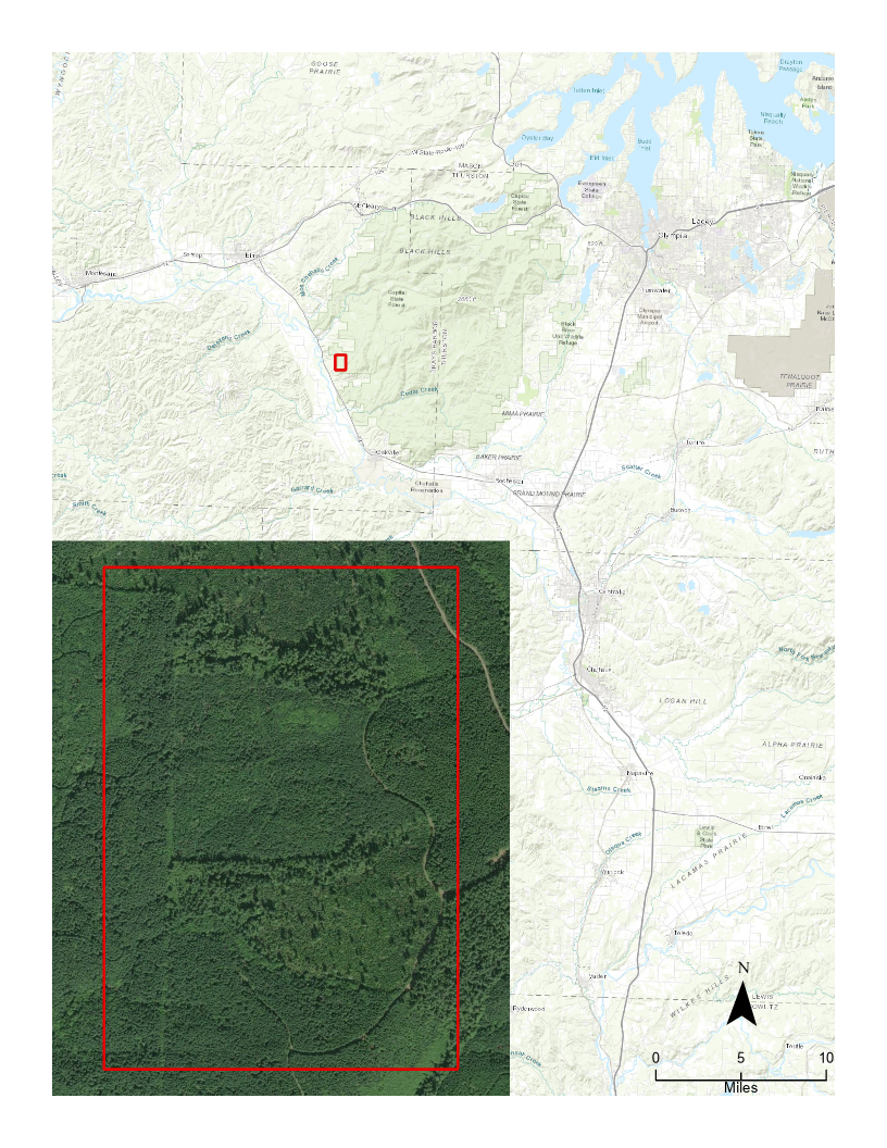
The data for this analysis covers a section of the Capitol State Forest, which is southwest of Olympia, Washington (see Figure 3). This forest is managed by the Washington State Department of Natural Resources and is used primarily as a resource for timber and recreation, but also naturally serves as carbon storage (Ear to the Ground, 2019). The LiDAR data was downloaded from the Washington State Department of Natural Resources Washington LiDAR Portal. This section of the forest was surveyed in 2012, so the data is eight years old. Because timber harvest occurs frequently in this forest, data from 2012 likely will not reflect the forest’s current metrics. However, resolution was 10.94 points per square meter, which exceeded the target of 8 points per square meter and was filtered to remove inaccurate points (Martinez, 2012).
Results
The analysis for this project resulted in two rasters: canopy cover and tree height. To create the canopy cover raster, I followed ESRI’s Estimating forest canopy density and height tutorial. To use the LiDAR data, the point cloud LAZ needed to be converted to LAS format. This was accomplished using an open source software called LASzip. Next, the data was separated into ground (class 2) and vegetation (classes 1, 3, 4, and 5) layers, including all return types, using the Make LAS Dataset Layer tool in ArcGIS Pro. The layers were converted to rasters and null values converted to equal zero. Finally, the ground raster was divided by the sum of the ground and vegetation rasters to find the vegetation density above ground (see Figure 4). In order to find the total canopy cover percentage for the area of interest, this raster was converted to integer format, an attribute table was built for the layer, and field calculator was used to calculate the percent of cells containing vegetation.
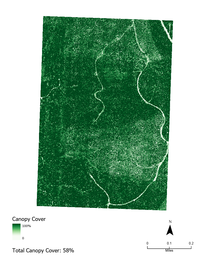
Figure 4
To create the tree height raster, I followed Earth Lab’s Canopy Height Models, Digital Surface Models & Digital Elevation Models – Work With LiDAR Data in Python tutorial. To complete this step, I downloaded the DSM and DTM data from the Washington LiDAR Portal for my area of interest. The measurement unit for this data was in feet. To create the raster, I simply used the Minus tool in ArcGIS Pro to subtract the DTM layer from the DSM layer. The output was a raster (see Figure 5) ranging in height from zero to 273 feet.
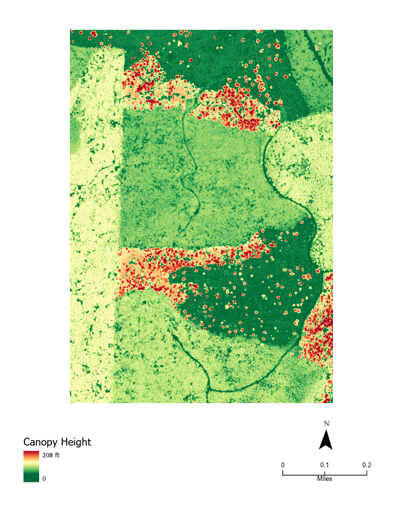
Figure 5
- Bonan, G. B. (2008). Forests and climate change: forcings, feedbacks, and the climate benefits of forests. Science, 320, 1444-1449. doi: 10.1126/science.1155121
- Ear to the Ground. (2019). Capitol forest didn’t always look so green.
- IPCC. (2014). Climate change 2014 synthesis report summary for policymakers.
- Martinez, D. (2012). LiDAR data acquisition and processing: Chehalis River watershed study area. Watershed Sciences, Inc.
- Stephens, P. R., Kimberley, M. O., Beets, P. N., Paul, T. S. H., Searles, N., Bell, A., Brack, C., & Broadley, J. (2012). Airborne scanning LiDAR in a double sampling forest carbon inventory. Remote Sensing of Environment, 117, 348-357. https://doi.org/10.1016/j.rse.2011.10.009
- Estimating forest canopy density and height tutorial
- Canopy Height Models, Digital Surface Models & Digital Elevation Models – Work With LiDAR
Data in Python tutorial